This post was expanded into a conference paper presented at AISTATS 2019: “On Multi-Cause Causal Inference with Unobserved Confounding: Counterexamples, Impossibility, and Alternatives” (https://arxiv.org/abs/1902.10286).
Last updated 2018-07-24.
Note: This post is the second in a series motivated by several recent papers about causal inference from observational data when there are multiple causes or treatments being assessed and there is unobserved confounding. See the first post here.
Goal
In observational causal inference, unobserved confounding is a constant threat to drawing valid causal inferences. If there are unobserved variables that affect both treatment assignment and outcomes, then one cannot, in general, precisely quantify causal relationships from observational data, even as the sample size goes to infinity.
Several recent papers have examined a special case of the unobserved confounding problem where it has been suggested that this identification problem might be solved. Specifically, they propose that if there are a large number of treatment factors, such that we can analyze the problem in the frame where the number of treatments goes to infinity, then the unobserved confounder may be consistently estimable from the data, and thus adjusted for like an observed confounder. I will call this strategy latent confounder reconstruction.
The purpose of this technical post is to highlight a central weakness of this strategy. In particular, if the latent variable is not degenerate and can be estimated consistently (in many cases it cannot), then the positivity assumption (defined below) will be violated with respect to that latent variable. Equivalently, if the positivity assumption holds with respect to the latent variable, then the latent variable cannot be estimated consistently.
The positivity assumption, also known as overlap or common support, is a necessary condition for doing causal inference without strong modeling assumptions. Thus, the result in this post implies that latent confounder reconstruction can only be used to estimate causal effects under strong parametric assumptions about the relationship between treatment, confounder, and outcome.
I’ll write this post in Pearl’s notation, using the do operator, but the translation to potential outcomes is straightforward.
Latent Confounder Reconstruction
Notation and Observed Confounders
We consider \(m\)-dimensional treatments \(X\), \(d\)-dimensional confounder \(Z\), and \(1\)-dimensional outcome \(Y\). The causal query of interest is the family of intervention distributions \[ P(Y \mid do(X)), \] or the family of distributions of the outcome \(Y\) when the treatments \(X\) are set to arbitrary values.
If \(Z\) were observed, the following assumptions would be sufficient to answer the causal query nonparametrically:
- Unconfoundedness: \(Z\) blocks all backdoor paths between \(X\) and \(Y\), and
- Positivity: \(P(X \in A \mid Z) > 0\), for each set \(A\) in the sample space of \(X\) for which \(P(X \in A) > 0\).
By the unconfoundedness asumption, the following relations hold: \[ P(Y \mid do(X)) = E_{P(Z)}[P(Y \mid X, Z)] = \int_{z \in \mathcal{Z}} P(Y \mid X, z) dP(z). \] Under the postivity assumption, all pairs of \((X, Z)\) are observable, so all terms of the rightmost expression can be estimated without parametric assumptions. Without the positivity assumption, the relations are still valid, but one needs to impose some parametric structure on \(P(Y \mid X, Z)\) so that this conditional distribution can be estimated for combinations of \((X, Z)\) that are not observable.
“Reconstructing” the Latent \(Z\)
In actuality, the confounder \(Z\) is not observed. Latent confounder reconstruction adds one additional assumption.
- Consistency: There exists some estimator \(\hat Z(X)\) such that, as \(m\) grows large \[\hat Z(X) \stackrel{a.s.}{\longrightarrow} Z.\]
The general idea is that if \(Z\) can be “reconstructed”" using a large number of observed treatments, then we should be able to adjust for the reconstructed \(Z\) in the same way we would have adjusted for \(Z\) if it were observed.
Here, I’m using strong consistency (almost-sure convergence) because the notation’s a bit more intuitive. This could be replaced with convergence in probability with a few more \(\epsilon\)’s.
Incompatibility with Positivity
Unfortunately, the very fact that the latent variable \(Z\) can be estimated consistently implies that the positivity assumption is violated as \(m \rightarrow \infty\).
The central idea is as follows: when \(\hat Z(X)\) is consistent, in the large \(m\) limit, the event \(Z=z\) implies that \(X\) must take a value \(x\) such that \(\hat Z(x) = z\). Thus, for distinct values of \(Z\), \(X\) must lie in distinct regions of the treatment space, violating positivity.
We show this formally in the following proposition.
When positivity is violated, we require strong modeling assumptions to fill in conditional distributions \(P(Y \mid X, Z)\) for pairs \((X, Z)\) that are unobservable. This is particularly difficult in the case of unobserved confounding because we are extrapolating a conditional distribution where one of the conditioning arguments is itself unobserved.
Example
Model
Consider the following example, with one-dimensional, binary latent variable \(Z\), and continuous treatments \(X\). In the structural model, we assume that the treatments are mutually independent of each other when \(Z\) is known, but that the variance of these treatments is four times as large when the latent variable \(Z = 1\) versus when \(Z = 0\). Further, we assume that the expectation of the outcome \(Y\) depends on the value of \(Z\) and whether the norm of the treatments \(\|X\|\) exceeds a particular threshold. \[ \begin{align} Z &\sim \text{Bern}(0.5)\\\\ X &\sim N_m(0, \sigma^2(Z) I_{m \times m})\\ \sigma(Z) &:= \left\{ \begin{array}{rl} \sigma &\text{if } Z = 0\\ 2\sigma &\text{if } Z = 1 \end{array} \right.\\\\ Y &\sim N(\mu(Z, X), 1)\\ \mu(Z,X) &:= \left\{ \begin{array}{rl} \alpha_{00} &\text{if } Z = 0 \text{ and }\|X\|/\sqrt{m} < 1.5\sigma\\ \alpha_{01} &\text{if } Z = 0 \text{ and } \|X\|/\sqrt{m} \geq 1.5\sigma\\ \alpha_{10} &\text{if } Z = 1 \text{ and }\|X\|/\sqrt{m} < 1.5\sigma\\ \alpha_{11} &\text{if } Z = 1 \text{ and }\|X\|/\sqrt{m} \geq 1.5\sigma \end{array} \right. \end{align} \]
We will analyze this example as the number of treatmnet \(m\) goes to infinity.
Consistent Estimation of \(Z\)
First, note that as the number of treatments \(m\) grows large, the latent variable \(Z\) can be estimated perfectly for any unit. Writing \(X = (X^{(1)}, \cdots, X^{(m)})\), by the strong law of large numbers \[ \sqrt{\frac{\sum_{j = 1}^m {X^{(j)}}^2}{m}} = \|X\|/\sqrt{m} \stackrel{a.s.}{\longrightarrow} \sigma(Z_i). \] From this fact, we con construct consistent esitmators \(\hat Z(X)\) for \(Z\). For example, letting \(I\{\cdot\}\) be an indicator function, \[\hat Z(X) := I\{\|X\|/\sqrt{m} > 1.5\sigma\}\] is consistent as \(m\) grows large.
We can visualize this example with a polar projection of the random vector \(X\) at various values of \(m\). This is one of my favorite visualizations, inspired by Figure 3.6 in Roman Vershynin’s High Dimensional Probability (pdf). We represent a vector of treatments \(X\) using polar coordinates, where the radius is given by \(\|X\|/\sqrt{m}\) and the angle is given by the angle that \(X\) makes with an arbitrary 2-dimensional plane (because the distribution of \(X\) is spherically symmetric the choice of the plane does not matter). This repressentation highlights a well-known concentration of measure phenomenon, where high-dimensional Gaussian vectors concentrate on a shell around the mean of the distribution.
In the figure, I’m plotting 1000 draws of the treatment vector \(X\) under each of the latent states \(Z = 0\) and \(Z = 1\) when \(m\) takes the values \(\{2, 20, 200\}\). We also plot the boundary where \(\hat Z(X)\) changes value from 0 to 1 (that is, where \(\|X\|/\sqrt{m}\) crosses \(1.5\sigma\)). It is evident that as \(m\) grows large, the cases where \(Z=0\) and \(Z=1\) are clearly separated by this boundary, and thus, \(\hat Z(X)\) is consistent as \(m\) grows large.
require(mvtnorm)## Loading required package: mvtnorm# 2-D polar coordinates to cartesion coordinates
polar2cartesian <- function(r, ang){
cbind(r*cos(ang), r*sin(ang))
}
# Plot 2-D polar projection of high-dimensional spherical Gaussians from model
# with decision boundary for Zhat
plot_polar_proj <- function(sig, m=100, n=1e3, decision=1.5, ...){
x0 <- rmvnorm(n, rep(0,m), diag(sig^2, m))
x1 <- rmvnorm(n, rep(0,m), diag((2*sig)^2, m))
# Polar projection of high-dimensional vector.
proj_coords <- function(x1){
d1 <- c(1, rep(0, m-1))
d2 <- c(0, 1, rep(0, m-2))
proj <- cbind(d1, d2)
x1p <- x1 %*% proj
norm1 <- sqrt(rowSums(x1^2)/m)
raw_dir <- acos(x1p[,1]/sqrt(x1p[,1]^2+x1p[,2]^2))
dir1 <- ifelse(x1p[,2] > 0, raw_dir, 2*pi-raw_dir)
cbind(norm1*cos(dir1), norm1*sin(dir1))
}
p0 <- proj_coords(x0)
#p0_normed <- t(apply(p0, 1, function(r){ r / sqrt(sum(r^2)) * 1.5 * sig}))
p1 <- proj_coords(x1)
boundary <- polar2cartesian(1.5*sig, seq(0, 2*pi, length.out=50))
ps <- rbind(p0, p1)#,
#p0_normed)
col0 <- 'red'
col1 <- 'blue'
plot(ps[,1], ps[,2], col=c(rep(col0, n), rep(col1,n)), pch=46, cex=2,
xlab=NA, ylab=NA, main=sprintf("m = %d", m), ...)
lines(boundary[,1], boundary[,2])
}
par(mfrow=c(1, 3), mar=c(2,2,2,2), bty='n')
lims <- c(-3, 3)
plot_polar_proj(1, m=2, ylim=lims, xlim=lims)
plot_polar_proj(1, m=20, ylim=lims, xlim=lims)
plot_polar_proj(1, m=200, ylim=lims, xlim=lims)
legend('bottomright', c("Z = 0", "Z = 1", expression(hat(Z)~boundary)), col=c("red", "blue", "black"), pch=c(46, 46, NA), lty=c(NA, NA, 1), bty='o', box.col='white', bg="#00000011", pt.cex=8)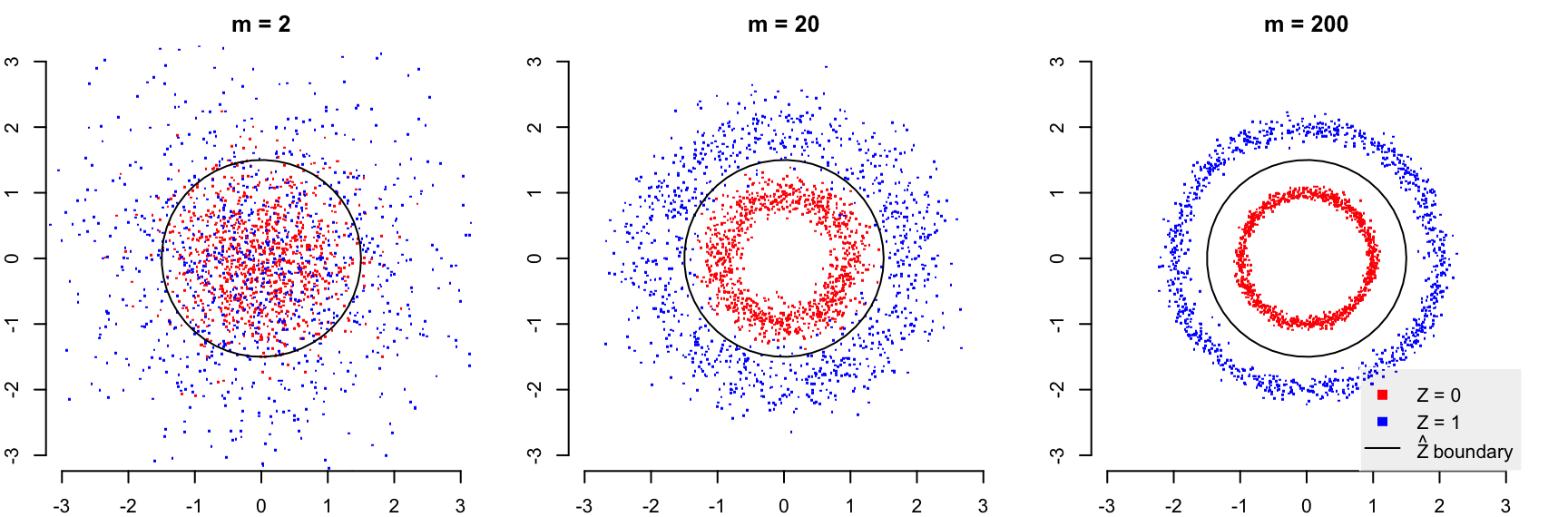
Plot of polar projection of treatments \(X\), colored by the value of the latent confounder \(Z\). As \(m\), the dimension of \(X\), increases, the treatment vectors \(X\) generated under each value of \(Z\) become more distinct. We take advantage of this distinctness to estimate \(Z\) consistently; as \(m\) grows large, the black boundary encodes an estimator \(\hat Z(X)\) that calls \(Z=0\) if a point lands inside the circle, and \(Z=1\) if it lands outside. However, this separation between red and blue points also indicates a positivity violation. To view a larger version of this image, try right-clicking and opening the image in a new tab.
Unobservable Expectations
Because \(\hat Z(X)\) is a consitent esitmator, certain conditional probability distributions \(P(Y \mid X, Z)\) cannot be estimated from the data. In particular, as \(m\) grows large, the probability of observing outcomes informing the following two parameters falls to zero: \[ \alpha_{01} = E[Y \mid Z = 0, \hat Z(X) = 1]\\ \alpha_{10} = E[Y \mid Z = 1, \hat Z(X) = 0], \] because the probability of observing pairings \((X, Z)\) such that \(\hat Z(X) \neq Z\) falls to zero. Thus, the mean of \(Y\) in the structural model, \(\mu(X, Z)\), cannot be estimated from the data in these two cases.
To see this from the figure above, note that the expected outcome \(\mu(X, Z)\) for each unit in the figure is a function of the point’s color and whether it lies on the inside or outside of the black circle. As \(m\) grows large, we only observe red points inside the circle and blue points outside; the probability of observing an outcome corresponding to, say, a red point outside of the circle, falls to zero.
In this case, any query \(P(Y \mid do(X))\) cannot be completed, unless one makes additional modeling assumptions about how these parameters are related to the identified parameters \(\alpha_{00}\) and \(\alpha_{11}\).
Takeaways
Given that there is a fundamental incompatibility between positivity and reconstructing latent confounders, what can be done? We either need to live without the positivity assumption, or change the way we attempt to identify causal effects when latent confounding is present.
The only way to proceed without positivity is to make parametric modeling assumptions about the structural model for \(Y\). We might assume, for example, that \[ \mu(X, Z) = \alpha X + \beta Z \] for some coefficient vectors \(\alpha\) and \(\beta\). This linear, separable specification allows one to extrapolate \(\mu(X, Z)\) to combinations of \((X, Z)\) that are unobservable. Less restrictively, we might assume that \(Y\) only depends on statistics of \(X\) that are ancillary to \(Z\); if this is the case, then there would be perfect overlap in the functions of \(X\) that actually determine \(Y\). In the example above, the direction of \(X\) is independent of \(Z\), so if \(\mu(X, Z)\) only depended on the direction of \(X\) and not its magnitude, then the structural model for \(Y\) could still be estimated. 1
One can also consider cases where \(Z\) cannot be reconstructed with full precision. Given the identification relation from the intro section, to calculate \(P(Y \mid do(X))\), it is sufficient to recover the distributions \(P(Z)\) and \(P(Y \mid X, Z)\). We can do this without reconstructing \(Z\), although we require additional information to do so. This additional information can come in the form of proxies (e.g., in Miao et al 2017), or in the form of parametric assumptions about the distributions \(P(Z)\) and \(P(Y \mid X, Z)\). In the latter case, there is a rich literature on identification in mixture models (Hennig 2002 contains a short review).
In either case, identification of causal effects when unobserved confounding is present is incredibly hard. It is perhaps the central problem in all of observational causal inference. Sensitivity analysis may be a more fruitful approach if one suspects that this is a problem in a particular study. I discuss sensitivity analysis in slightly more detail in my last post on the multiple causal inference problem.
Thanks to Alex Franks and Uri Shalit for their feedback on this post. Thanks to Rajesh Rangananth for thoughtful comments on the first post on latent confounders; these comments inspired this post.
This ancillarity assumption is equivalent to assuming that \(\hat Z(X)\) is a proxy (variable that is causally downstream of \(Z\) but conditionally independent of \(Y\)), so this approach would be similar to the proxy identification strategy discussed in the next paragraph.↩